I am trying to keep myself updated with the LLM literature and recently found an interesting course from HuggingFace that covers a practical introduction to LLM alignment. It is very useful because the course is designed so you can run everything on your machine with minimal hardware requirements. After checking some of the content, I started going into a loop of papers, blog posts, and documentation. So, I decided to start writing this post to use as notes in the future. I hope anyone else finds it useful too.
Table of contents
- What is preference alignment?
- PPO: Proximal Policy Optimization
- DPO: Direct Preference Optimization
- ORPO: Monolithic Preference Optimization without Reference Model
What is preference alignment?
Training a large language model (LLM) can involve several steps:
- Train model on next token prediction: This is done on a massive amount of data since we do not need to do any kind of labeling. Raw text is enough, we just need to predict the next token in a sequence and backpropagate the error.
- Supervised fine-tuning (SFT): This is the step where we fine-tune the model to a specific task. This can be a chatbot, a summarizer, a translator, etc. We need labeled data for this step.
- Preference Aligment: Force the model to follow a specific set of rules or preferences. Like do not using offensive language, do not generate fake news, etc.
Nowadays, the first step is done by companies with access to massive amounts of data and computational resources such as Anthropic, OpenAI, Meta, etc. We usually refer to these as Base Models, and those that have been fine-tuned to follow a specific task as Instruct Models. See, for example, Qwen/Qwen2-7B and Qwen/Qwen2-7B-instruct.
A simple example of a dataset used for supervised fine-tuning can be a chatbot dataset like the one below:
| Prompt | Response |
|---|---|
| What is Celta de Vigo stadium? | Celta de Vigo’s stadium is Balaídos. |
| Who is Celta de Vigo’s most popular player? | The most popular and iconic player in the history of Celta de Vigo is Iago Aspas. |
A simple example of model alignment is to provide our fine-tuned chatbot model with a prompt and two different responses: one that aligns with our preferences and one that does not. The goal is to train the model to prefer the response that aligns with our preferences. Check for example the Ultrafeedback dataset in HuggingFace datasets.
Gathering this kind of data can be very expensive and time-consuming. Fine-tuning involves a prompt and a single response, while alignment requires a prompt and multiple responses. We need to define how to rank these replies (good/bad).
Let’s explore the different methods we can use to align our models!
PPO
Proximal Policy Optimization is a Reinforcement Learning (RL) algorithm that iteratively improves the model’s policy while maintaining stability. This might sound complex, but the idea is simple. In RL, an agent interacts with an environment by taking actions. These actions change the environment, and the agent receives rewards based on the outcomes of its actions. The goal is to learn a policy that maximizes the expected reward.
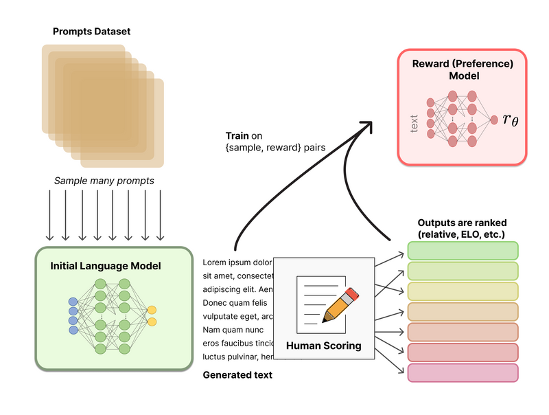
In the context of LLMs, the agent is the model, the state is the input prompt, and the action is the generated response. We need a reward model to evaluate the quality of these responses. While we could use human feedback for this, having humans intervene in the training loop is impractical. Instead, we can train a model to provide feedback on the responses as a human would. This model is called a reward model.
Figure 1. Diagram showing the pipeline to train a reward model (obtained from HuggingFace blog)
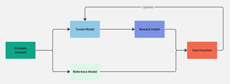
Once we have a reward model we can plugin it in our RL training loop and use the PPO algorithm to train our model. See the diagram below:
Figure 2. Diagram showing the PPO pipeline
Initially, both the tuned model and the reference model are identical copies of our starting SFT model. PPO uses the reference model to ensure that the tuned model does not exploit the reward model by generating responses that score well but are irrelevant (think of a chatbot that always responds with “I don’t know”). The reward model, which has been previously trained on human feedback, evaluates responses based on how well they align with our desired preferences.
The RL objective for this task is generally expressed as:
\[\begin{equation} J_{\text{RLHF}} = \max_{\pi_\theta} \mathbb{E}_{x \sim D, y \sim \pi_\theta(y|x)} \left[ r_\varphi(x, y) - \beta \mathbb{D}_{KL} \left[ \pi_\theta(y|x) \| \pi_{\text{ref}}(y|x) \right] \right] \end{equation}\]Where $\pi_{\theta}$ is the policy/model we are trying to learn, $D$ is the dataset of prompts and responses, $r_{\varphi}$ is the reward model, $\beta$ is a hyperparameter that controls the trade-off between maximizing the reward and minimizing the KL divergence term. The KL divergence is in charge of keeping the policy close to the reference model to avoid exploitation.
Have in mind that is not possible to apply gradient descent directly to this objective. The variable \(y\sim \pi_\theta(y\|x)\) is sampled from our LLM and this involes non-differentiable operations (check this post to learn more about the different sampling methods).
PPO has proven to be a very effective algorithm for alignin LLMs but it is also a complex and often unstable procedure. What if we could simplify this process?
DPO
Direct Preference Optimization (DPO) is a recent work from 2023 that won an outstanding paper award at NeurIPS. The main idea of this work is to remove RL from the alignment process, as it introduces complexity, instability, and the need for a reward model.
Instead, we can directly optimize our SFT model to generate responses that align with our preferences. In the previous section, we saw that the cost function could not be optimized directly because of the non-differentiable sampling operation, but DPO solves this problem elegantly.
Mathematical derivation
We start with an SFT model that we need to align with a dataset of preferences, denoted as \(y_w \succ y_l \mid x\), where $y_w$ and $y_l$ represent the preferred and dispreferred responses, respectively. These preference are assumed to be generated by some latent reward model $r^*(x, y)$ which we do not have access to. We can convert these preferences into a score using the Bradley-Terry model:
\[P(y_w > y_l) = \frac{e^{r^*(x, y_w)}}{e^{r^*(x, y_w)} + e^{r^*(x, y_l)}}\]We can then use Maximum Likelihood Estimation (MLE) to estimate the parameters of a reward model $r_{\theta} (x, y)$ that maximizes this probability. For doing this we start by rewriting the Bradley-Terry model as a sigmoid expression:
\[\sigma(A - B) = \frac{1}{1 + e^{-(A - B)}} = \frac{e^{A - B}}{1 + e^{A - B}} = \frac{e^A}{e^A + e^B}\]Note that the right side of our equation is equivalent to the Bradley-Terry model. So if rewrite Eq. 2 by using the sigmoid function we get:
\[\mathcal{L}_R(r_\theta, D) = -\mathbb{E}_{(x,y_w,y_l)\sim D}\left[\log \sigma (r_\theta(x, y_w)) - r_\theta(x, y_l)\right]\]Note that we have added a log term to the sigmoid function to avoid numerical instability and a negative sign to convert the maximization problem into a minimization one.
Why is this useful? Because we can directly train a model with this loss function, which will learn to assign higher scores to preferred responses. The reward model for this setting is generally initialized from the SFT model we started with, but with an extra linear layer on top that produces the score.
It is known that the optional solution for Eq. 1 under a general reward function $r$ is given by:
\[\pi_r(y|x) = \frac{1}{Z(x)} \pi_{ref}(y|x) \exp \left( \frac{1}{\beta} r(x,y) \right)\]where $Z(x) = \sum_y \pi_{ref}(y|x) \exp \left( \frac{1}{\beta} r(x,y) \right)$. The only problem is that this is not computationally feasible because of the Z term that involves generating all possible responses $y$ for the given prompt $x$ (that is every sentence you can build with the vocabulary of the model).
Now is when the magic happens. Let’s assume we have access to the optimal policy $\pi^*(y|x)$. If we replace it in the previous equation and solve for $r(x,y)$ by applying the logarithm to both sides, we get:
\[r(x,y) = \beta \log \frac{\pi^*(y|x)}{\pi_{ref}(y|x)} + \beta \log Z(x)\]This means that if we could get the optimal policy, we could use that to obtain a reward model… And that is where the Bradley-Terry model comes into play. Pay attention to this since it is the key idea of DPO! Combining Eq. 2 and Eq. 3 we get:
\[P(y_{w} > y_l) = \sigma(r(x, y_w) - r(x, y_l))\]If we now update the latest equation with our reward model (Eq. 6) we just get:
\[P(y_{w} > y_l) = \sigma \left( \beta \log \frac{\pi^*(y_w|x)}{\pi_{ref}(y_w|x)} + \beta \log Z(x) - \beta \log \frac{\pi^*(y_l|x)}{\pi_{ref}(y_l|x)} - \beta \log Z(x) \right)\]And that’s how the Z term cancels out! See that we have moved from defining preferences in terms of the reward model to defining them in terms of the optimal policy. We can just maximize our previous expression or minimize the negative version of it. This is the loss function we will use to train our model:
\[L_{DPO}(\pi_{\theta}; \pi_{ref}) = -\mathbb{E}_{(x, y_w, y_l) \sim D} \left[ \log \sigma \left( \beta \log \frac{\pi_{\theta}(y_w | x)}{\pi_{ref}(y_w | x)} - \beta \log \frac{\pi_{\theta}(y_l | x)}{\pi_{ref}(y_l | x)} \right) \right]\]This is just awesome.
TLDR
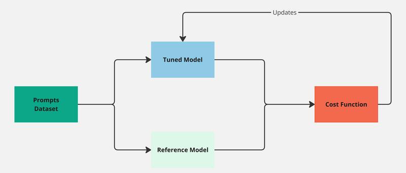
This section became larger than expected, but in summary, we can say that DPO provides a way to remove RL from the alignment process. We can directly train our SFT model with a dataset of preferences using the loss function derived in the previous section. Gradient descent is all we need now, and our alignment diagram simplifies to:
Figure 3. Diagram showing the DPO pipeline
HuggingFace team compared DPO with other aligning methods that I am not covering in this post (IPO and KTO). It showed
HuggingFace team compared DPO with other alignment methods (IPO and KTO) and found that DPO performed the best, followed by KTO, and then IPO. Check their blog post for more details.
ORPO
Monolithic Preference Optimization without Reference Model proposes a new method that directly integrates the alignment step in the SFT phase. This removes the need of a reference model anymore reducing the number of steps in our training pipeline. It is a very simple and powerful idea. Let’s follow the paper explanation and start from how the SFT loss function is defined:
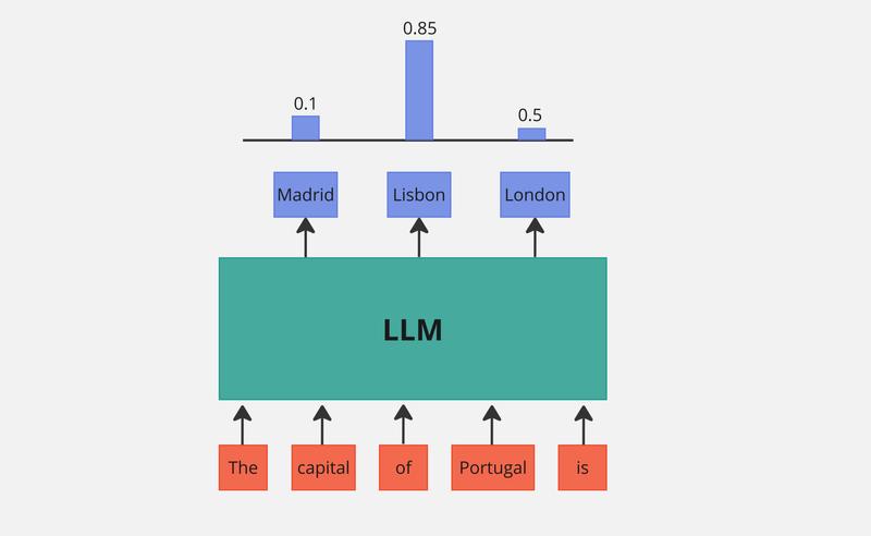
\[\log P_{\theta}(y|x) = \frac{1}{m} \sum_{t=1}^{m} \log P_{\theta}(y_t|x, y_{<t})\]This loss basically tries to make the log-likelihood of the output tokens as high as possible given the input prompt. The diagram below shows a intuitive representation of this process:
Figure 4. LLM Diagram
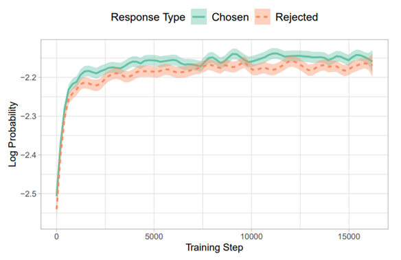
The goal of this loss function is to maximize the probability of the correct next word (Lisbon) given the previous words (The capital of Portugal is). This loss focuses on maximizing the likelihood of the correct token and does not directly penalize incorrect tokens (Madrid, London). When aligning a language model, we use a dataset of preferences with chosen and rejected responses (as seen in the HF dataset). The absence of a penalty for incorrect responses can result in these rejected responses sometimes having a higher likelihood than the chosen ones! The next figure shows an example of this:
You might be guessing what this paper is going to propose… and yes! It introduces a penalty term for the rejected responses. Let’s start by defining how likely it is for our model $\theta$ to generate an output sequence:
\[\mathcal{L}_{ORPO} = \mathbb{E}_{(x, y_w, y_l)}[\mathcal{L}_{SFT} + \lambda \cdot \mathcal{L}_{OR}]\]With this simple equation we can compute the odds for the model to generate the preferred response over the dispreferred one:
\[OR_{\theta}(y_w, y_l) = \frac{odds_{\theta}(y_w|x)}{odds_{\theta}(y_l|x)}\]This is converted into a loss function by wrapping the log odds ratio with the log sigmoid function. The logs are used to avoid numerical instability, and the sigmoid maps the log odds ratio to a probability. The authors explore the gradient of this loss in the paper, providing justification for its use.
The final loss function is comprised of two terms, the SFT loss and the OR loss:
\[\mathcal{L}_{ORPO} = \mathbb{E}_{(x, y_w, y_l)} [\mathcal{L}_{SFT} + \lambda \cdot \mathcal{L}_{OR}]\]ORPO is computationally more efficient than the previous methods and it is also achieves better results (check the experiments section of the paper). The diagram below shows the simplified ORPO pipeline:
Figure 5. Diagram showing the ORPO pipeline. Note it uses the Base Model instead of starting from a SFT trained one.
There is also a very interesting post from HuggingFace team that shows how they have used ORPO for training Llama3 and obtained very encouraging results. You can check it here.
References
- [1] Schulman, J., Wolski, F., Dhariwal, P., Radford, A., & Klimov, O. (2017). Proximal policy optimization algorithms. arXiv preprint arXiv:1707.06347.
- [2] Rafailov, R., Sharma, A., Mitchell, E., Manning, C. D., Ermon, S., & Finn, C. (2024). Direct preference optimization: Your language model is secretly a reward model. Advances in Neural Information Processing Systems, 36.
- [3] Hong, J., Lee, N., & Thorne, J. (2024, November). Orpo: Monolithic preference optimization without reference model. In Proceedings of the 2024 Conference on Empirical Methods in Natural Language Processing (pp. 11170-11189).
- [4] LLM Alignment
- [5] Direct Preference Optimization (DPO) explained
- [6] HF Alignment Handbook
- [7] HF blog post on RLHF
